|
|
| ||||||
in a previous post, we counted the number of aligned sequences that overlapped with a list of genes using htseq. here, we will show how to do the same thing using the genomic ranges bioconductor package.
to get started, first download the aligned sequence reads and the genomic annotation set provided on this blog post. the data is a subset of the data found in the pasilla bioconductor package.
next, open up R and install the genomic ranges package:
we are now ready to use genomic ranges to generate a list of counts per per gene.
to get started, first download the aligned sequence reads and the genomic annotation set provided on this blog post. the data is a subset of the data found in the pasilla bioconductor package.
wget http://www.weebly.com/uploads/2/6/8/5/26850053/aligned.bamthe aligned sequence reads are stored in a binary sequencing alignment/map format, and the genomic annotation set is in the gtf format.
wget http://www.weebly.com/uploads/2/6/8/5/26850053/chr4.gtf.gz
next, open up R and install the genomic ranges package:
 source("http://bioconductor.org/biocLite.R")
biocLite("GenomicRanges", dependencies=TRUE)
we will also need rsamtools and rtracklayer. source("http://bioconductor.org/biocLite.R")
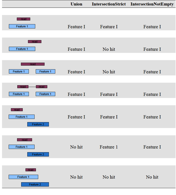
biocLite(c("Rsamtools", "rtracklayer", "GenomicAlignments"), dependencies=TRUE) just like htseq, genomic ranges includes three overlap resolution modes that dictate how aligned reads that overlap more than one genomic feature are treated. the three overlap resolutions modes are { union, intersection-strict, intersection-nonempty }. union only counts reads that overlap any portion of exactly one feature (i.e., reads that overlap multiple features are discarded); intersection-strict only counts reads which fall completely within only one feature (.e.g, if a feature has coordinates 1-10, and the read overlaps coordinates 6-11, the read is not counted for that feature, since the read exceeds the coordinates of the feature); and, lastly, intersection-nonempty only counts reads that fall within a unique disjoint region of a feature (in the case of partially overlapping features, if a read overlaps with at least one base that is unique to one of the features, the read is counted for that feature). a figure depicting these overlap resoltuons modes is available here. for a full list of genomic ranges counting options, consult the vignette.we are now ready to use genomic ranges to generate a list of counts per per gene.
library(GenomicRanges)the output is a table in the same format as htseq. examine the first five lines of the output file in R using head in the system command:
library(GenomicAlignments)
library(Rsamtools)
library(rtracklayer)
gtf <- import("chr4.gtf.gz", # import gtf file
asRangedData=FALSE) # return GRanges object instead of a RangedData obj
idx <- mcols(gtf)$type == "exon" # find lines in gtf that are exons only
exons <- gtf[idx] # create table composed of only exons
genes <- split(exons, mcols(exons)$gene_name) # split by by gene name
params <- ScanBamParam( # set bam file params
flag=scanBamFlag(isUnmappedQuery=FALSE), # only consider mapped reads
tag="NH") # include NH tag, which reports if each read maps uniquely
bam <- readGAlignments("aligned.bam", # read bam file
param=params) # include params
unique_hits <- bam[mcols(bam)$NH == 1] # remove multimapping reads
counts <- summarizeOverlaps( # summarize overlaps function
features=genes, # count reads per gene
reads=unique_hits, # the data to be counted
mode="Union", # use the union mode
ignore.strand=TRUE, # data is not stranded
SingleEnd=TRUE, # data is single-end
param=params)
count_table <- assays(counts, withDimnames=TRUE)$counts # create table of counts
write.table(count_table, # write the count table to disk
file="aligned.granges.counts", # save as file name 'aligned.granges.counts'
sep = "\t", # outut as tab delimited
row.names=TRUE, # include the row (gene) names in output
col.names=FALSE, # don't write column names
quote=F) # don't place double quotes around factor or characters
 system("head -n 5 aligned.granges.counts")
# Actbeta       0
# Ank   6750
# Arf102F       0
# Asator        205
# ATPsyn-beta   0
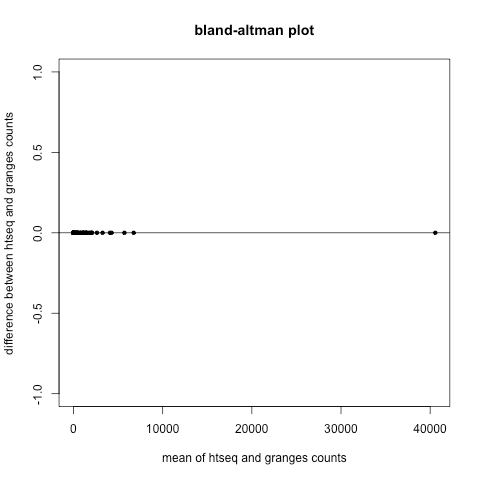
to see how the counting from htseq compares to genomic ranges, we can make a bland-altman plot (also know as a 'mean-difference plot'). htseq_file <- "http://www.weebly.com/uploads/2/6/8/5/26850053/aligned.htseq.counts"a bland-altman plot measures the degree of agreement between two measurements. as can be see, there is no difference between counts per gene as measured by htseq and counts per gene as measured by genomic ranges, that is, the counts per gene as determined by htseq are equivalent to the counts per gene as determined by genomic ranges.
htseq_counts <- head(read.table(file=htseq_file, # read htseq count file
sep='\t', # the file is tab delimited
header=FALSE, # the file has no header
row.names=1, # the first column is the row (gene) names
col.names=c("gene", "count")), # provide columnn names
-5) # remove the last 5 lines, which are htseq special counters
granges_counts <- read.table(file="aligned.granges.counts", # read genomic ranges count file
sep='\t',
header=FALSE, # plot x=mean, y=difference
row.names=1,
col.names=c("gene", "count"))
htseq_sorted <- htseq_counts[order(row.names(htseq_counts)),] # sort the htseq count file by row (gene) name
granges_sorted <- granges_counts[order(row.names(granges_counts)),] # sort the genomic ranges count file by row (gene) name
md.plot <- function(x,y, xlab="mean", # create a bland-altman function with defaults
ylab="difference",main="bland-altman plot") {
mean <- (x+y)/2 # mean between x and y
difference <- x-y # difference between x and y
plot(mean, difference, # plot the mean vs the difference
xlab=xlab,
ylab=ylab,
main=main, # the plot title
pch=20) # point type as solid
abline(h=0) # draw a horizontal line at y=0
}
md.plot(htseq_sorted, granges_sorted, # plot the mean-difference between the htseq and genomic ranges counts
xlab="mean of htseq and granges counts", # x-axis label
ylab="difference between htseq and granges counts") # y-axis label


 RSS Feed